Goals
The goal of this lab was to gain experience in the measurement and interpretation of spectral reflectance signatures of various Earth surface and near surface materials captured by satellite images. Additionally, we explored performing basic monitoring of Earth resources using remote sensing band ratio techniques. For this lab, the study area was Eau Claire County and Chippewa County in Wisconsin.
Methods
All exercises in this lab were completed using Erdas Imagine 2015 and ArcMap 10.3.1.
Spectral Signature Analysis
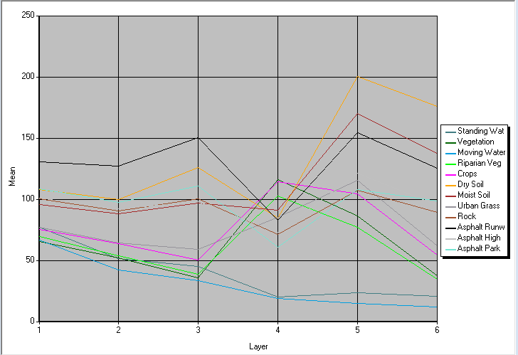
During the first part of this lab, we measured and plotted the spectral reflectances of 12 different surface features from a satellite image of Eau Claire in Erdas Imagine. These materials included moving water, vegetation, dry soil, etc. To locate the desired surface, I linked my Erdas Imagine Viewer to Google Earth (Figure 1). Then, upon finding the desired surface, I utilized the Polygon tool to draw a square around the surface and opened the Signature Editor to view the polygon area's spectral signature mean plot. After collecting the spectral reflectances of all 12 surfaces, I displayed all of the spectral reflectance signature mean plots together and completed analysis (Figure 2). Differences between materials can be detected when examining their spectral reflectance signature mean plots; for example, when taking a look at the curves for dry and moist soil, there are clear discrepancies (Figure 3). Dry soil shows an overall higher amount of reflectance due to its lesser moisture content, while moist soil displays lower reflectance levels due to its higher moisture content.
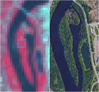 |
Figure 1: spectral reflectance signature collection process for riparian vegetation;
Erdas Imagine (left), Google Earth (right) |
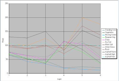 |
| Figure 2: all spectral reflectance signatures |
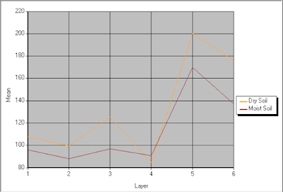 |
| Figure 3: spectral reflectance signature mean plot for dry and moist soil |
Resource Monitoring
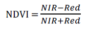 |
| Figure 4: NDVI ratio |
The second part of this lab involved resource monitoring of vegetation health and soil health through performing simple band ratios. Firstly, we utilized Erdas Imagine to implement the normalized difference vegetation index (NDVI) on an image of Eau Claire County and Chippewa County to determine abundance of vegetation. This involved using the NDVI function within Erdas Imagine, which carried out the NDVI ratio (Figure 4). This produced a black and white NDVI image, with extremely white areas indicating high levels of vegetation and darker areas indicating less vegetation (Figure 5). I then imported this image into ArcMap and created a map of vegetation health (Figure 8).
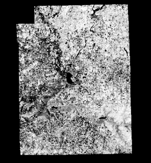 |
| Figure 5: NDVI image viewed in Erdas Imagine |
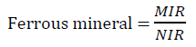 |
| Figure 6: ferrous mineral ratio |
Next, I utilized Erdas Imagine to implement the ferrous mineral ratio on an image of Eau Claire County and Chippewa County to determine the spatial distribution of iron contents in soils within this area. This involved using the Indices function under the Unsupervised tab in the Raster section of Erdas Imagine, which carried out the ferrous mineral ratio (Figure 6). This produced a black and white image, with lighter areas depicting areas of ferrous minerals and darker areas showing areas with less amounts of such minerals (Figure 7). I then imported this image into ArcMap and created a map of soil health (Figure 9).
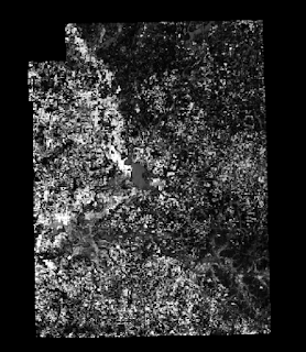 |
| Figure 7: ferrous mineral map viewed in Erdas Imagine |
Results
Below are the results of my methods, namely two maps depicting vegetation and soil health (Figure 8, 9). As these maps show, carrying out simple band ratio analysis can be very helpful in monitoring Earth resources. Such data may be especially useful to farmers or the DNR in terms of gauging the health of various landscapes and determining future plans of action.
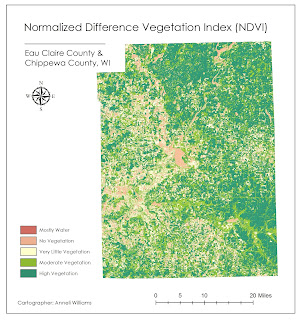 |
| Figure 8: map displaying vegetation health |
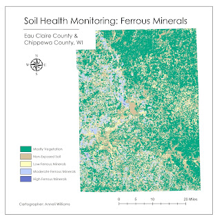 |
| Figure 9: map displaying soil health |
Sources
Satellite image is from Earth Resources Observation and Science Center, United States Geological Survey.


No comments:
Post a Comment