Lab 6: Geometric Correction

Goals

The purpose of this lab was to provide an introduction to an important image preprocessing exercise, namely geometric correction.  Geometric correction is performed on satellite images as a part of preprocessing activities prior to the extraction of biophysical and sociocultural information from the images.  There are two major types of geometric correction, image-to-map rectification and image-to-image registration, both of which were explored in this lab.  

Methods

Image-to-Map Rectification: 
During the first part of this lab, I geometrically corrected an image using image-to-map rectification in Erdas Imagine 2015.  To do this, I first opened both the image to be rectified and the reference image in Erdas Imagine.  Then, I navigated to raster processing tools for multispectral imagery and used the Control Points function to begin the geometric correction process.  After this, I set the geometric model to Polynomial.  For this exercise, I ran a 1st order polynomial transformation.  

Then, I began to the process of adding Ground Control Points (GCPs) to both of the images using the Create GCP tool. The number of required GCPs varies depending on the extent of geometric distortion present in an image; moderate distortion only requires affine (linear) transformation and fewer GCPs while more serious geometric distortion requires higher order polynomial transformation and more GCPs (Figure 1).  Since this exercise involved a 1st order polynomial transformation, a minimum of 3 pairs of GCPs were necessary.  For this lab, however, I added four pairs of GCPs.  After adding the third pair of GCPs, the model solution changed from reading "model has no solution" to "model solution is current" because the necessary number of GCPs was achieved.  When adding points, I tried to place them in distinctive locations that could be easily found on both the image to be rectified and the reference map.  I also tried to evenly disperse my GCPs throughout the images.  

After placing all four pairs of GCPs, I evaluated their accuracy by examining the Root Mean Square (RMS) error.  The total RMS error is indicated in the lower right hand corner of the Multipoint Correction Window.  The ideal RMS error is .5 and below, however, for this lab, mine only needed to be below 2.0.  To achieve this, I made small adjustments to my GCPs' locations until my error dipped below 2.0 (Figure 2).  Once my total RMS error had been reduced, I performed the geometric correction using the Natural Neighbor resampling method by clicking the Display Resample Image Dialog button.  This created a rectified output image (Figure 4).

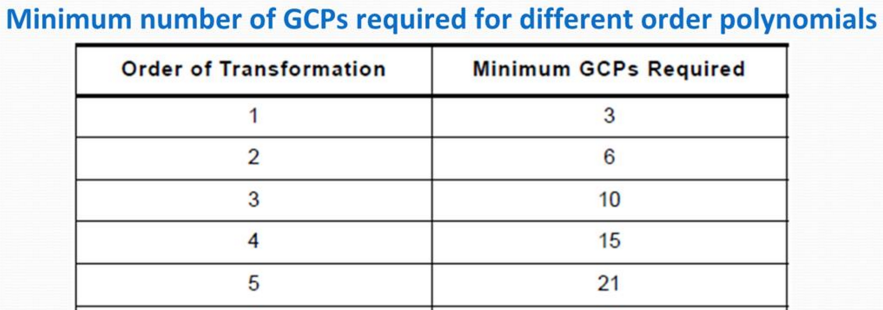
Figure 1: table indicating GCP requirement for different order polynomials

Figure 2: image-to-map registration geometric correction process in Erdas Imagine;
image to be rectified is on the left and reference map is on the right; RMS total error = .7275

Image-to-Image Registration: 

During this part of the lab, I geometrically corrected an imaged using image-to-image registration in Erdas Imagine 2015.  This involved essentially the same process that I outlined above for image-to-map rectification, except this time I used a previously rectified image for a reference instead of a map.  For this exercise, I performed a 3rd order polynomial transformation, so a minimum of 10 GCPs were required, though I added 12 GCPs.  After adding all 12 GCP pairs, I once again evaluated my geometric accuracy by assessing the RMS total error.  Upon achieving a total RMS error under 1.0, I moved on to the geometric correction process.  This time, I used the Bilinear Interpolation resampling method to geometrically correct the image by clicking the Display Resample Image Dialog button.  This produced a rectified output image (Figure 5).  

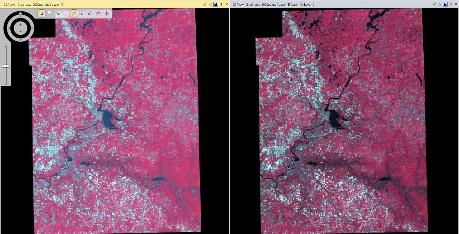
Figure 3: image-to-image registration geometric correction process in Erdas Imagine; 
image to be rectified is on the left and reference image is on the right

Results

The results of my methods are displayed below. 

Image-to-Map Rectification: 

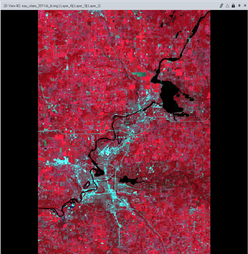
Figure 4: unrectified image on left; rectified image on right

Image-to-Image Registration: 

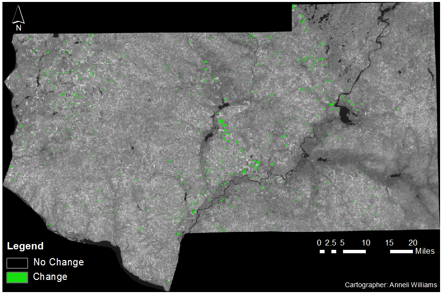
Figure 5: unrectified image on right; rectified image on left

Sources

Satellite images. Earth Resources Observation and Science Center, United States Geological Survey. 

Digital raster graphic (DRG) from Illinois Geospatial Data Clearing House. 

Lab 5: LiDAR

Goals

LiDAR (Light Detection and Ranging) is one of the recently expanding areas in remote sensing, with the accompanying skill set of dealing with LiDAR data becoming increasingly marketable.  In light of this, the purpose of this lab was to gain a basic understanding of LiDAR data structure and processing.  This involved working with LiDAR point clouds in LAS file format to carry out a number of exercises, including:  

• Processing and retrieval of various surface & terrain models
• Processing and creation of intensity image and other derivative products from point cloud

Methods

All exercises in this lab were completed using Erdas Imagine 2015 and ArcMap 10.3.1.

Part 1: Point Cloud Visualization in Erdas Imagine
In this part of the lab, we displayed all of the provided LAS files for the Eau Claire region in Erdas Imagine (Figure 1).  Had there been any overlapping points at the boundaries of tiles, they would have been removed at this point.  After viewing all of the LAS files together, I also examined the relevant metadata.  We completed all further analysis and manipulation of the data in ArcGIS because it has easier workflows in comparison with the point cloud tools in Erdas Imagine.  

Figure 1: LiDAR point cloud of Eau Claire County visualized in Erdas Imagine

Part 2: Generation of LAS Dataset & Exploration with ArcGIS

After opening the tile index and LAS files in ArcGIS, I completed the following: 

• Creation of a LAS dataset
• Exploration of the LAS dataset properties
• Visualization of the LAS dataset as point cloud in 2D and 3D

After creating the LAS dataset and assigning it an appropriate projection, I began to explore different ways of displaying the data.  The LAS Dataset Toolbar in ArcMap provides many different functions to aid in this, including viewing the data by Elevation, Aspect, Slope and Contour as well as applying a number of filters (Figure 2).  There is also the option of viewing the data with a 3D profile view, which can be very useful (Figure 3).

Figure 2: collage displaying LiDAR data viewed by Contour, Aspect, and Elevation respectively (left to right)

Figure 3 : 3D profile view of point cloud data in ArcMap

Part 3: Generation of LiDAR Derivative ProductsWhile LAS point cloud data is sufficient for visualization purposes, most applications require the creation of derivative products such as digital terrain models (DTM) and digital surface models (DSM).  In this part of the lab, I created four such derivative products:

• Digital Surface Model (DSM) with first return
• Digital Terrain Model (DTM)
• Hillshade of DSM
• Hillshade of DTM

First, to determine the spatial resolution at which the derivative products should be produced at, I took a look at the LAS dataset properties and estimated the average nominal pulse spacing (NPS) at which the point clouds were collected.  Then, I set the points to be displayed by elevation and set the filter to First Returns.  After this, I used the 'LAS to Raster' tool with the following parameters: Interpolation = Binning, Cell Assignment Type = Maximum, Void Fill Method = Natural_Neighbor, Sampling Type = Cell Size, Sampling Value = 6.56168 (approx. 2m) to create a DSM (Figure 3).  Then, I enhanced my DSM image by creating a hillshade of my first derivative product.  This process involved using the 'Hillshade' tool, found under 3D Analyst Tools, Raster Surface (Figure 4).  

Next, using the same  'LAS to Raster' tool, I derived a DTM from the LiDAR point cloud, setting the points to be displayed by elevation and filter to Ground.  In the tool, I used the following parameters: Interpolation = Binning, Cell Assignment Type = Minimum, Void Fill Method = Natural_Neighbor, Sampling Type = Cell Size, Sampling Value = 6.56168 (approx. 2m).  This DTM is a bare-Earth raster (Figure 5). Then, to create an image that showed more details about the Earth surface, I created a hillshade of my DTM using the 'Hillshade' tool (Figure 6).  

Finally, I created a LiDAR intensity image using a similar procedure as outlined above.  First, I set the LAS dataset to be displayed by elevation, with the filter set to First Returns.  I used First Returns since intensity is always captured by the first return echoes.  Then, I utilized the 'LAS to Raster' again with the following parameters: Value Field = Intensity, Interpolation = Binning, Cell Assignment Type = Average, Void Fill Method = Natural_Neighbor, Sampling Type = Cell Size, Sampling Value = 6.56168 (approx. 2m).  The resulting image appeared rather dark when displayed in ArcMap, so I viewed it in Erdas Imagine (Figure 7).  

Results

The results of my methods are displayed below. 

DSM & DSM Hillshade
The digital surface model (DSM) below (Figure 4) was created using LiDAR first returns.  It displays a generalized image of Eau Claire, with larger features discernible.  I also created a grayscale DSM Hillshade (Figure 5), which enhances the landscape by adding shaded relief to the features.  

  

Figure 4: DSM viewed in ArcMap

Figure 5: DSM Hillshade viewed in ArcMap

DTM & DTM Hillshade
The digital terrain model (DTM) below (Figure 6) displays very generalized topographic features of Eau Claire.  In contrast to the DSM above, this image does not display objects on the ground surface such as buildings or plants.  I also created a grayscale DTM Hillshade (Figure 7) which enhances the DTM image with relief shading. 

Figure 6: DTM viewed in ArcMap

Figure 7: DTM Hillshade viewed in ArcMap

Intensity Image

The intensity image below (Figure 8) depicts the intensity, or strongest return strength of the laser pulse, of each point for my Eau Claire LiDAR data.  Displaying images by their intensity values can aid in feature identification and in LiDAR point classification.  

Figure 8: Intensity Image viewed in Erdas Imagine 2015

Sources

Lidar point cloud and Tile Index are from Eau Claire County, 2013. 

Eau Claire County Shapefile is from Mastering ArcGIS 6th Edition data by Margaret Price, 2014.

Lab 4: Miscellaneous Image Functions

Goal and Background

The purpose of this lab was to provide an introduction to a number of image functions and exercises including exploration into the following: 

• image preprocessing
• image enhancement for visual interpretation
• delineation of study area from larger satellite image
• image mosaicking
• graphical model creation

Methods

All exercises in this lab were carried out using Erdas Imagine 2015, with images and files provided by Dr. Cyril Wilson. 

Part 1: Image Subsetting

The first part of this lab addressed two ways to subset images, a process very helpful in image interpretation.  Often times, a desired area of interest (AOI) will be smaller than the image at hand.  In these cases, it is advantageous to employ image subsetting to cut away the areas which fall outside of your area of interest.  

Image Subsetting Methods:

I. Inquire Box: The first subsetting method I tackled was utilizing an Inquire Box in Erdas Imagine to indicate my desired AOI and subset the image (Figure 1).  One disadvantage to this method is that the AOI produced will always be a rectangle, although your actual AOI may have a more irregular shape.  

Figure 1: image subsetting using the Inquire Box

II. Shapefile: The second subsetting method I tried out in Erdas Imagine involved using a shapefile for AOI delineation (Figure 2).  After overlaying the shapefile atop the original image, I used the Subset & Chip tool to complete the subsetting.  With this method, the image produced reflects the extent of the AOI regardless of its shape, making this method more suitable for irregular AOI areas than the first method.  

Figure 2: image subsetting using shapefile of AOI

Part 2: Image Fusion
Sometimes, an image is not the spatial resolution that one desires.  In these cases, pansharpening, or the use of a panchromatic band to enhance the spatial resolution of a multispectral image, can be helpful.  In this lab, I loaded the original image and panchromatic image into Erdas Imagine, noting that the images had spatial resolutions of 30m and 15m respectively.  I then used the Resolution Merge tool to carry out the pansharpening process.  The resulting pansharpened image clearly possessed a higher spatial resolution than the original image, with features appearing much more defined.


Part 3: Radiometric Enhancement

When collecting images, one cannot assure that there will be perfect atmospheric conditions.  Sometimes, occurrences such as haze can negatively impact the quality of images.  Luckily, radiometric enhancement techniques can help combat this and increase image quality.  In this lab, I utilized the Haze Reduction tool to reduce the effects of haze upon an image, thus making it easier to complete image interpretation (Figure 4).  

Part 4: Linking Image Viewer to Google Earth
Recent versions of Erdas Imagine have allowed for a handy function called Google Earth Linking.  This allows the user to sync images loaded into Erdas Imagine with images on Google Earth, providing for simultaneous zooming in/out of the same areas (Figure 3).  In this way, Google Earth imagery stands as a form of a selective image interpretation key. 

Figure 3: Google Earth Linking displaying image in Erdas and in Google Earth

Part 5: Image Resampling
Image resampling refers to the process of changing the size of pixels, whether it be increasing or decreasing.  There are multiple methods of carrying out this process including Nearest Neighbor, Bilinear Interpolation, Cubic Convolution, and Bicubic Spline.  Each of these methods has various advantages and disadvantages and is suited to different purposes.  

In this lab, I utilized first utilized Nearest Neighbor to resample an image from 30m to 15m (output image: Figure 12).  While this method did work, it produced an image that was not much higher quality than the original image.  When zoomed in, a pixelated "stairstepped" effect was visible around curves and diagonals.  

Next, I resampled the same image using Bilinear Interpolation (output image: Figure 13).  In comparison to the resampled image produced using Nearest Neighbor, this output image was much smoother.  When zoomed in, curves and diagonals did not display a "stairstepped" effect (Figure 4).  

Figure 4: closer look at Bilinear Interpolation smoother resampling around curves

Part 6: Image Mosaicking
Image mosaicking is the process of stitching multiple satellite images together to form one, larger image.  This process is helpful when the desired AOI is larger than the extent of just one satellite image, or when the AOI falls along the boundary between two satellite images.  There are two different ways of mosaicking an image in Erdas Imagine, Mosaic Express and MosaicPro.  

In this lab, I first mosaicked two images together using Mosaic Express.  This process was quick and easy, however, the resulting image was not a smoothly stitched image (Figure 14).  The color transition at the boundary between both images was quite jarring, and the image as a whole was not cohesive.  

After this, I used MosaicPro to stitch the same two satellite images together.  This method required considerably more user input in regards to color correction, overlay functions, etc.  The resulting image was much more cohesive than the previous one, and had a smooth color transition at the boundary between the two images (Figure 15).  

Part 7: Image Differencing
Image differencing, also known as binary change detection, involves analyzing pixel brightness to determine changes in landscapes over time.  In this process, the pixel brightness values of an image taken at one date are subtracted from that of another image taken at a earlier or later date.  These two images must have the same radiometric characteristics and identical spatial, spectral, and temporal resolution.  The results of image differencing are displayed as a Gaussian histogram.

In this exercise, the study area was Eau Claire county and four of its surrounding counties.  Two images of this area were used, with one from 1991 and the other from 2011.  To carry out the image differencing process, I utilized Model Maker in Erdas Imagine (Figure 5).  Then, I analyzed the resulting Gaussian histogram using a graphic provided by my instructor (Figure 6, Figure 7).  Finally, I created a map in ArcGIS depicting areas of change within the AOI (Figure 12). 

Figure 5: Model Maker equation used to carry out Image Differencing

Figure 6: Gaussian histogram; result of image differencing

Figure 7: graphic explaining Gaussian histogram analysis

Results

The results of my methods are displayed below. 

Image Subset:

Figure 8: image subset produced with Inquire Box method

Figure 9: image subset produced by AOI delineation with shapefile

Image Fusing:

Figure 10: original image (left) vs. pan-sharpened image (right)

Haze Reduction:

Figure 11: original image (left) and haze reduced image (right)

Image Resampling:

Figure 12: resampling using Nearest Neighbor; original image (left), resampled image (right)

Figure 13: resampling using Bilinear Interpolation; original image (left), resampled image (right)

Image Mosaicking:

Figure 14: result of Mosaic Express

Figure 15: result of MosaicPro

Image Differencing:

Figure 16: map depicting areas of landscape change in the Chippewa Valley 1991 - 2011

Conclusion

This lab exposed me to lots of image functions that are essential for image interpretation.  The manipulation of an image depends on the goals of the project at hand and the properties of the image itself.  Image functions can be used in combination with each other to achieve the best possible image for interpretation.  No image is completely perfect, but with the aid of these processes, image interpretation can be improved.   

Sources

Satellite images from Earth Resources Observation and Science Center, United States Geological Survey.

Shapefile from Mastering ArcGIS 6th edition Dataset by Maribeth Price, McGraw Hill. 2014.